Dataset containing the initial number of susceptible and infected cattle (individuals) across three age categories in 1,600 herds (nodes). Provides a heterogeneous population structure for demonstrating SISe3 model simulations in a compartmental modeling context.
Usage
data(u0_SISe3)Details
This dataset represents initial disease states in a synthetic population of 1,600 cattle herds (nodes) stratified into three age categories. Each row represents a single herd (node). The SISe3 model extends the SISe model with age-structured compartments (S_1, I_1, S_2, I_2, S_3, I_3) and an environmental compartment for pathogen shedding. This is appropriate for diseases where transmission rates or recovery rates differ by age group.
The data contains:
- S_1
Total susceptible cattle (individuals) in age category 1 in the node
- I_1
Total infected cattle in age category 1 (initialized to zero)
- S_2
Total susceptible cattle in age category 2
- I_2
Total infected cattle in age category 2 (initialized to zero)
- S_3
Total susceptible cattle in age category 3
- I_3
Total infected cattle in age category 3 (initialized to zero)
The herd size distribution and age structure is synthetically generated to reflect heterogeneity typical of large-scale populations, making it suitable for illustrating how to incorporate scheduled events in the SimInf framework.
See also
SISe3 for creating SISe3 models with this initial
state and events_SISe3 for associated cattle
movement and demographic events
Examples
## For reproducibility, call the set.seed() function and specify the
## number of threads to use. To use all available threads, remove the
## set_num_threads() call.
set.seed(123)
set_num_threads(1)
## Create an 'SISe3' model with 1600 cattle herds (nodes) stratified
## by age, initialize it to run over 4*365 days and record data at
## weekly time-points. Add ten infected animals to age category 1 in
## the first herd to seed the outbreak. Define 'tspan' to record the
## state of the system at weekly time-points. Load scheduled events
## events for the population of nodes with births, deaths and
## between-node movements of individuals.
u0 <- u0_SISe3
u0$I_1[1] <- 10
model <- SISe3(
u0 = u0,
tspan = seq(from = 1, to = 4*365, by = 7),
events = events_SISe3,
phi = rep(0, nrow(u0)),
upsilon_1 = 1.8e-2,
upsilon_2 = 1.8e-2,
upsilon_3 = 1.8e-2,
gamma_1 = 0.1,
gamma_2 = 0.1,
gamma_3 = 0.1,
alpha = 1,
beta_t1 = 1.0e-1,
beta_t2 = 1.0e-1,
beta_t3 = 1.25e-1,
beta_t4 = 1.25e-1,
end_t1 = 91,
end_t2 = 182,
end_t3 = 273,
end_t4 = 365,
epsilon = 0
)
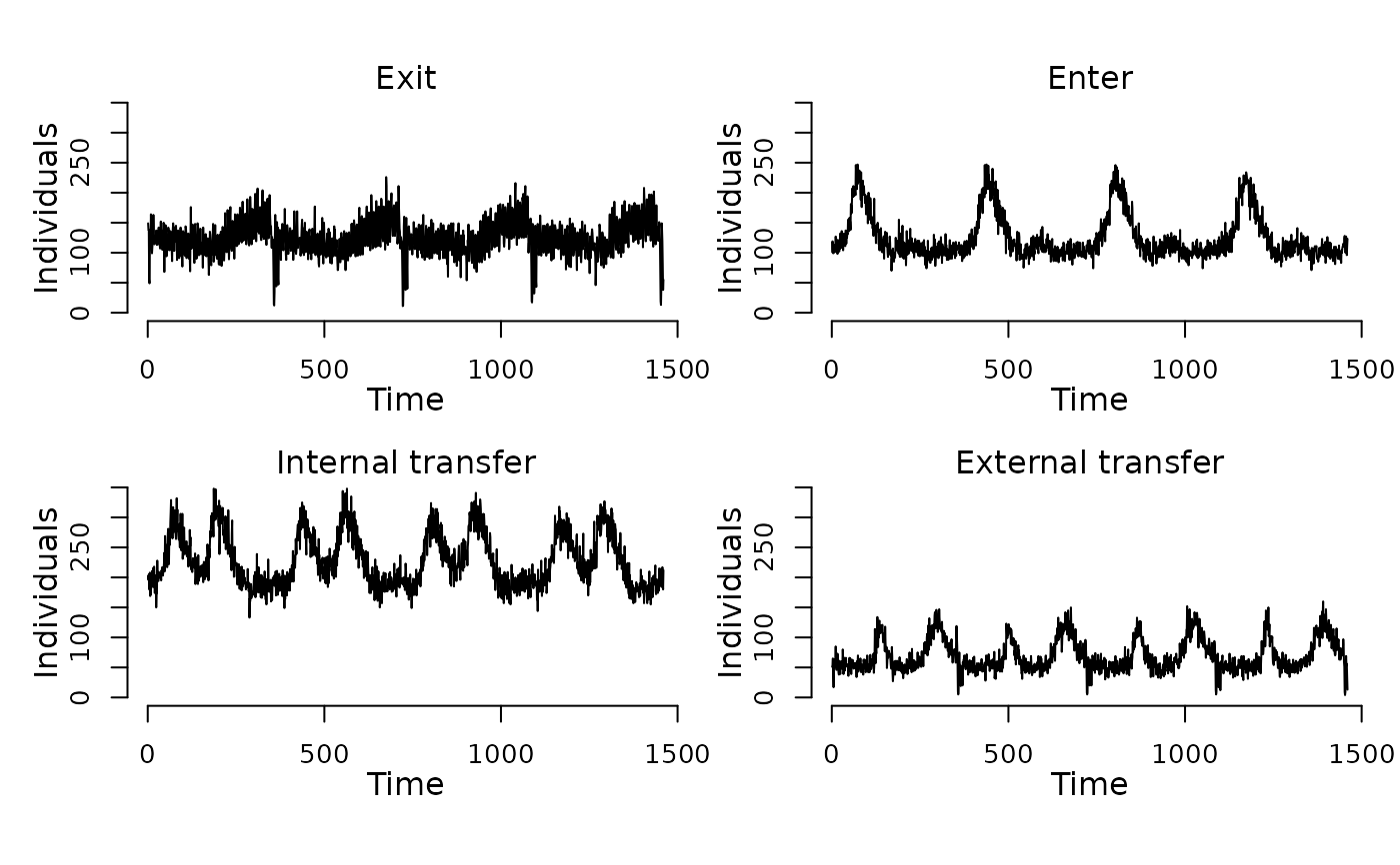
## Display the number of cattle affected by each event type per day.
plot(events(model))
 ## Run the model to generate a single stochastic trajectory.
result <- run(model)
## Plot the median and interquartile range of the number of
## susceptible and infected individuals.
plot(result)
## Run the model to generate a single stochastic trajectory.
result <- run(model)
## Plot the median and interquartile range of the number of
## susceptible and infected individuals.
plot(result)
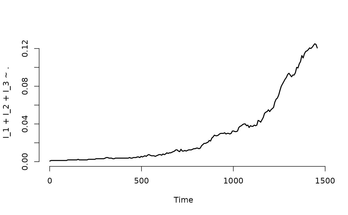
 ## Plot the proportion of nodes with at least one infected individual.
plot(result, I_1 + I_2 + I_3 ~ ., level = 2, type = "l")
## Plot the proportion of nodes with at least one infected individual.
plot(result, I_1 + I_2 + I_3 ~ ., level = 2, type = "l")
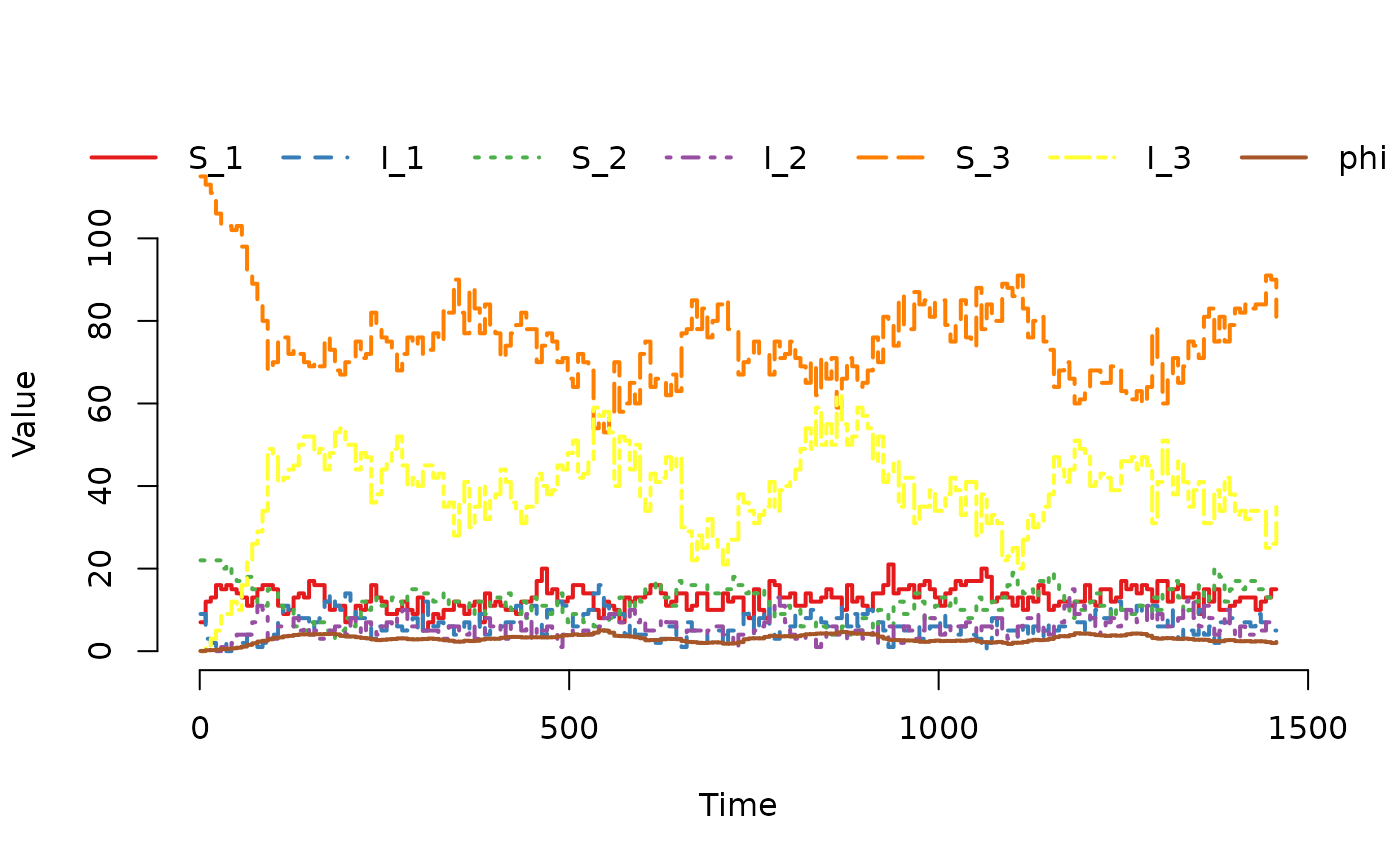
 ## Plot the trajectory for the first herd.
plot(result, index = 1)
## Plot the trajectory for the first herd.
plot(result, index = 1)
 ## Summarize the trajectory. The summary includes the number of events
## by event type.
summary(result)
#> Model: SISe3
#> Number of nodes: 1600
#>
#> Transitions
#> -----------
#> S_1 -> upsilon_1*phi*S_1 -> I_1
#> I_1 -> gamma_1*I_1 -> S_1
#> S_2 -> upsilon_2*phi*S_2 -> I_2
#> I_2 -> gamma_2*I_2 -> S_2
#> S_3 -> upsilon_3*phi*S_3 -> I_3
#> I_3 -> gamma_3*I_3 -> S_3
#>
#> Global data
#> -----------
#> Parameter Value
#> upsilon_1 0.018
#> upsilon_2 0.018
#> upsilon_3 0.018
#> gamma_1 0.100
#> gamma_2 0.100
#> gamma_3 0.100
#> alpha 1.000
#> beta_t1 0.100
#> beta_t2 0.100
#> beta_t3 0.125
#> beta_t4 0.125
#> epsilon 0.000
#>
#> Local data
#> ----------
#> Parameter Value
#> end_t1 91
#> end_t2 182
#> end_t3 273
#> end_t4 365
#>
#> Scheduled events
#> ----------------
#> Exit: 182535
#> Enter: 182685
#> Internal transfer: 317081
#> External transfer: 101472
#>
#> Network summary
#> ---------------
#> Min. 1st Qu. Median Mean 3rd Qu. Max.
#> Indegree: 40.0 57.0 62.0 62.1 68.0 90.0
#> Outdegree: 36.0 57.0 62.0 62.1 67.0 89.0
#>
#> Continuous state variables
#> --------------------------
#> Min. 1st Qu. Median Mean 3rd Qu. Max.
#> phi 0.0000 0.0000 0.0000 0.0524 0.0000 5.7011
#>
#> Compartments
#> ------------
#> Min. 1st Qu. Median Mean 3rd Qu. Max.
#> S_1 0.0000 7.0000 9.0000 9.1710 11.0000 30.0000
#> I_1 0.0000 0.0000 0.0000 0.0561 0.0000 16.0000
#> S_2 0.0000 14.0000 18.0000 17.8635 22.0000 43.0000
#> I_2 0.0000 0.0000 0.0000 0.1104 0.0000 18.0000
#> S_3 0.0000 74.0000 94.0000 96.7399 118.0000 206.0000
#> I_3 0.0000 0.0000 0.0000 0.5943 0.0000 83.0000
## Summarize the trajectory. The summary includes the number of events
## by event type.
summary(result)
#> Model: SISe3
#> Number of nodes: 1600
#>
#> Transitions
#> -----------
#> S_1 -> upsilon_1*phi*S_1 -> I_1
#> I_1 -> gamma_1*I_1 -> S_1
#> S_2 -> upsilon_2*phi*S_2 -> I_2
#> I_2 -> gamma_2*I_2 -> S_2
#> S_3 -> upsilon_3*phi*S_3 -> I_3
#> I_3 -> gamma_3*I_3 -> S_3
#>
#> Global data
#> -----------
#> Parameter Value
#> upsilon_1 0.018
#> upsilon_2 0.018
#> upsilon_3 0.018
#> gamma_1 0.100
#> gamma_2 0.100
#> gamma_3 0.100
#> alpha 1.000
#> beta_t1 0.100
#> beta_t2 0.100
#> beta_t3 0.125
#> beta_t4 0.125
#> epsilon 0.000
#>
#> Local data
#> ----------
#> Parameter Value
#> end_t1 91
#> end_t2 182
#> end_t3 273
#> end_t4 365
#>
#> Scheduled events
#> ----------------
#> Exit: 182535
#> Enter: 182685
#> Internal transfer: 317081
#> External transfer: 101472
#>
#> Network summary
#> ---------------
#> Min. 1st Qu. Median Mean 3rd Qu. Max.
#> Indegree: 40.0 57.0 62.0 62.1 68.0 90.0
#> Outdegree: 36.0 57.0 62.0 62.1 67.0 89.0
#>
#> Continuous state variables
#> --------------------------
#> Min. 1st Qu. Median Mean 3rd Qu. Max.
#> phi 0.0000 0.0000 0.0000 0.0524 0.0000 5.7011
#>
#> Compartments
#> ------------
#> Min. 1st Qu. Median Mean 3rd Qu. Max.
#> S_1 0.0000 7.0000 9.0000 9.1710 11.0000 30.0000
#> I_1 0.0000 0.0000 0.0000 0.0561 0.0000 16.0000
#> S_2 0.0000 14.0000 18.0000 17.8635 22.0000 43.0000
#> I_2 0.0000 0.0000 0.0000 0.1104 0.0000 18.0000
#> S_3 0.0000 74.0000 94.0000 96.7399 118.0000 206.0000
#> I_3 0.0000 0.0000 0.0000 0.5943 0.0000 83.0000