Post-process data in a trajectory

After a model is created, a simulation is started with a call to the run() function. The function returns a modified model object containing a single stochastic solution trajectory. This trajectory includes the state of each compartment recorded at every time-point specified in tspan.

This vignette introduces the functionality in SimInf to post-process and explore this trajectory data.

Let us first load the SimInf package.

library(SimInf)

Extract trajectory data with `trajectory()`

Most modeling studies require custom data analysis beyond simple plotting. To support this, SimInf provides the trajectory() method to extract the raw data as a data.frame. This is useful if you need to:

Perform custom statistical calculations (e.g., time to peak).
Export data to CSV for use in other software.
Combine results from multiple simulation runs.

Let’s simulate 10 days of data from an SIR model with 6 nodes. For reproducibility, we set the seed and specify the number of threads.

set.seed(123)
set_num_threads(1)

u0 <- data.frame(
  S = c(100, 101, 102, 103, 104, 105),
  I = c(1, 2, 3, 4, 5, 6),
  R = c(0, 0, 0, 0, 0, 0)
)

model  <- SIR(
  u0 = u0,
  tspan = 1:10,
  beta = 0.16,
  gamma = 0.077
)

result <- run(model)

Extract the full trajectory data (all compartments, all nodes).

trajectory(result)

##    node time   S  I R
## 1     1    1 100  1 0
## 2     2    1 101  2 0
## 3     3    1 102  3 0
## 4     4    1 102  5 0
## 5     5    1 103  6 0
## 6     6    1 105  6 0
## 7     1    2 100  1 0
## 8     2    2 101  2 0
## 9     3    2 101  4 0
## 10    4    2 101  5 1
## 11    5    2 103  6 0
## 12    6    2 105  6 0
## 13    1    3  99  2 0
## 14    2    3 101  2 0
## 15    3    3 101  4 0
## 16    4    3  99  6 2
## 17    5    3 101  8 0
## 18    6    3 103  7 1
## 19    1    4  98  3 0
## 20    2    4 101  2 0
## 21    3    4 101  4 0
## 22    4    4  98  6 3
## 23    5    4  99 10 0
## 24    6    4 101  8 2
## 25    1    5  98  3 0
## 26    2    5 101  2 0
## 27    3    5 100  5 0
## 28    4    5  97  6 4
## 29    5    5  98  9 2
## 30    6    5 101  6 4
## 31    1    6  98  2 1
## 32    2    6 101  2 0
## 33    3    6 100  5 0
## 34    4    6  97  5 5
## 35    5    6  98  8 3
## 36    6    6 100  7 4
## 37    1    7  98  2 1
## 38    2    7  98  5 0
## 39    3    7 100  5 0
## 40    4    7  92 10 5
## 41    5    7  98  7 4
## 42    6    7  99  8 4
## 43    1    8  97  3 1
## 44    2    8  98  5 0
## 45    3    8  98  6 1
## 46    4    8  92  8 7
## 47    5    8  95 10 4
## 48    6    8  99  8 4
## 49    1    9  97  3 1
## 50    2    9  97  6 0
## 51    3    9  98  4 3
## 52    4    9  91  9 7
## 53    5    9  94 10 5
## 54    6    9  99  7 5
## 55    1   10  97  3 1
## 56    2   10  96  6 1
## 57    3   10  98  4 3
## 58    4   10  89 11 7
## 59    5   10  93  9 7
## 60    6   10  98  8 5

Extract the number of recovered individuals (R) in the first node only.

trajectory(result, compartments = "R", index = 1)

##    node time R
## 1     1    1 0
## 2     1    2 0
## 3     1    3 0
## 4     1    4 0
## 5     1    5 0
## 6     1    6 1
## 7     1    7 1
## 8     1    8 1
## 9     1    9 1
## 10    1   10 1

Extract the number of recovered individuals in the first and third nodes.

trajectory(result, compartments = "R", index = c(1, 3))

##    node time R
## 1     1    1 0
## 2     3    1 0
## 3     1    2 0
## 4     3    2 0
## 5     1    3 0
## 6     3    3 0
## 7     1    4 0
## 8     3    4 0
## 9     1    5 0
## 10    3    5 0
## 11    1    6 1
## 12    3    6 0
## 13    1    7 1
## 14    3    7 0
## 15    1    8 1
## 16    3    8 1
## 17    1    9 1
## 18    3    9 3
## 19    1   10 1
## 20    3   10 3

Calculate prevalence from a trajectory using `prevalence()`

The prevalence() function calculates the proportion of individuals with the disease. It takes a model object and a formula:

Left-hand side (LHS): Compartments representing “cases” (e.g., I).
Right-hand side (RHS): Compartments representing the “at-risk” population (e.g., S + I + R).

The function also supports a level argument to change the aggregation level:

level = 1 (default): Prevalence aggregated over all nodes (global).
level = 2: Proportion of nodes that have at least one case.
level = 3: Prevalence calculated within each node (returns a matrix).

Let’s determine the proportion of infected individuals in the total population.

prevalence(result, I ~ S + I + R)

##    time prevalence
## 1     1 0.03616352
## 2     2 0.03773585
## 3     3 0.04559748
## 4     4 0.05188679
## 5     5 0.04874214
## 6     6 0.04559748
## 7     7 0.05817610
## 8     8 0.06289308
## 9     9 0.06132075
## 10   10 0.06446541

Identical result is obtained with the shorthand I ~ . (where . means “all compartments”).

prevalence(result, I ~ .)

##    time prevalence
## 1     1 0.03616352
## 2     2 0.03773585
## 3     3 0.04559748
## 4     4 0.05188679
## 5     5 0.04874214
## 6     6 0.04559748
## 7     7 0.05817610
## 8     8 0.06289308
## 9     9 0.06132075
## 10   10 0.06446541

Calculate the proportion of nodes that are infected (at least one I individual).

prevalence(result, I ~ S + I + R, level = 2)

##    time prevalence
## 1     1          1
## 2     2          1
## 3     3          1
## 4     4          1
## 5     5          1
## 6     6          1
## 7     7          1
## 8     8          1
## 9     9          1
## 10   10          1

Calculate the prevalence within each node individually.

prevalence(result, I ~ S + I + R, level = 3)

##    node time prevalence
## 1     1    1 0.00990099
## 2     2    1 0.01941748
## 3     3    1 0.02857143
## 4     4    1 0.04672897
## 5     5    1 0.05504587
## 6     6    1 0.05405405
## 7     1    2 0.00990099
## 8     2    2 0.01941748
## 9     3    2 0.03809524
## 10    4    2 0.04672897
## 11    5    2 0.05504587
## 12    6    2 0.05405405
## 13    1    3 0.01980198
## 14    2    3 0.01941748
## 15    3    3 0.03809524
## 16    4    3 0.05607477
## 17    5    3 0.07339450
## 18    6    3 0.06306306
## 19    1    4 0.02970297
## 20    2    4 0.01941748
## 21    3    4 0.03809524
## 22    4    4 0.05607477
## 23    5    4 0.09174312
## 24    6    4 0.07207207
## 25    1    5 0.02970297
## 26    2    5 0.01941748
## 27    3    5 0.04761905
## 28    4    5 0.05607477
## 29    5    5 0.08256881
## 30    6    5 0.05405405
## 31    1    6 0.01980198
## 32    2    6 0.01941748
## 33    3    6 0.04761905
## 34    4    6 0.04672897
## 35    5    6 0.07339450
## 36    6    6 0.06306306
## 37    1    7 0.01980198
## 38    2    7 0.04854369
## 39    3    7 0.04761905
## 40    4    7 0.09345794
## 41    5    7 0.06422018
## 42    6    7 0.07207207
## 43    1    8 0.02970297
## 44    2    8 0.04854369
## 45    3    8 0.05714286
## 46    4    8 0.07476636
## 47    5    8 0.09174312
## 48    6    8 0.07207207
## 49    1    9 0.02970297
## 50    2    9 0.05825243
## 51    3    9 0.03809524
## 52    4    9 0.08411215
## 53    5    9 0.09174312
## 54    6    9 0.06306306
## 55    1   10 0.02970297
## 56    2   10 0.05825243
## 57    3   10 0.03809524
## 58    4   10 0.10280374
## 59    5   10 0.08256881
## 60    6   10 0.07207207

Visualize a trajectory with `plot()`

The plot() function provides a quick way to inspect the outcome. It can display:

The median and quantile range across all nodes.
Individual trajectories for specific nodes.
Prevalence curves.

Note: Since the simulation is stochastic, the exact lines shown below will vary unless set.seed() is used.

Aggregated View (Median and Range)

Plot the median and interquartile range (IQR) of all compartments.

plot(result)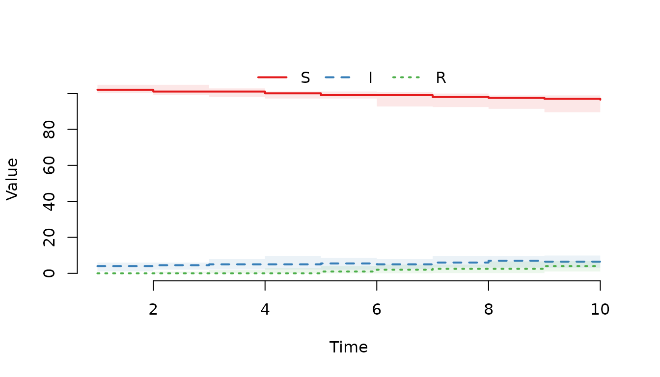

Plot the median and the middle 95% quantile range.

plot(result, range = 0.95)

Plot only the infected individuals (I).

plot(result, "I")

Use formula notation to plot the infected individuals.

plot(result, ~I)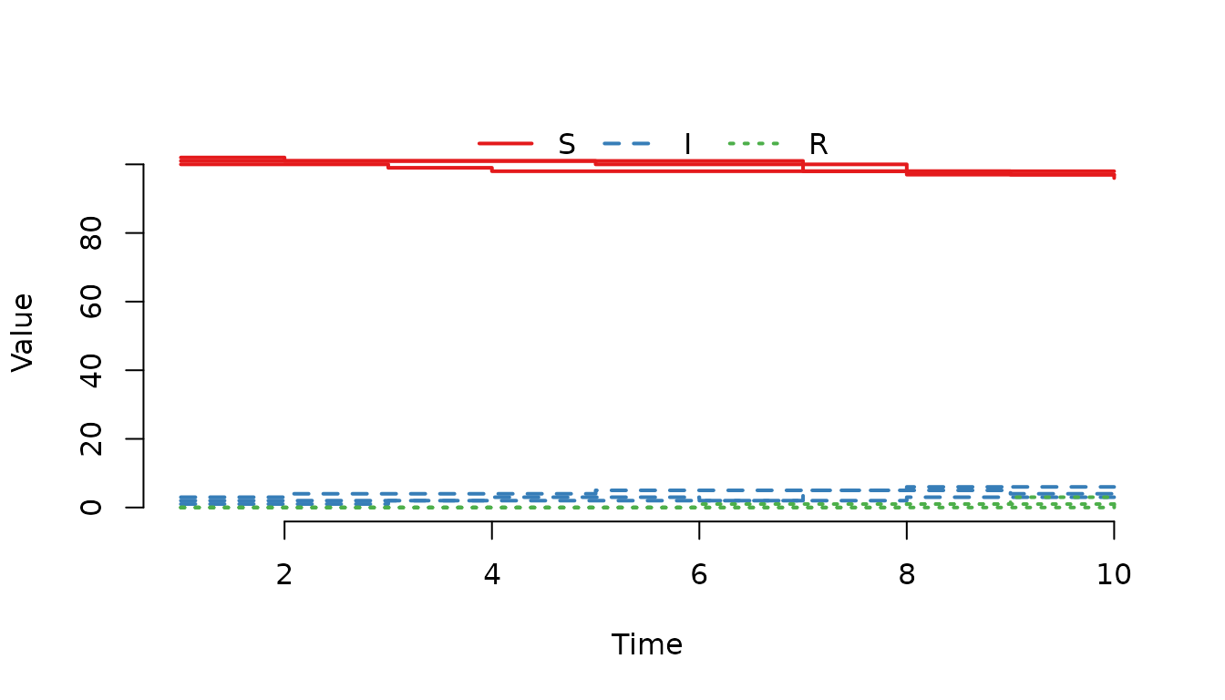

Individual Node View

Plot the trajectories for the first three nodes. We use range = FALSE to suppress the shaded median/range bands and show the individual lines.

plot(result, index = 1:3, range = FALSE)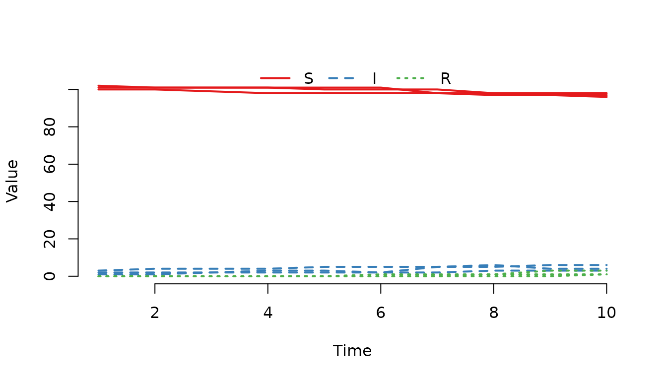

Use type = "l" to draw a line.

plot(result, index = 1:3, range = FALSE, type = "l")

Plot the infected individuals in the first node only.

plot(result, "I", index = 1, range = FALSE)

Prevalence Plots

Plot the proportion of infected individuals in the population.

plot(result, I ~ S + I + R)

Plot the proportion of nodes with infected individuals (level = 2).

plot(result, I ~ S + I + R, level = 2)

Plot the median and IQR of the prevalence within in each node (level = 3).

plot(result, I ~ S + I + R, level = 3)

Plot the prevalence in the first three nodes.

plot(result, I ~ S + I + R, level = 3, index = 1:3, range = FALSE)

Summary

Use trajectory() to extract raw data for custom analysis.
Use prevalence() to calculate disease proportions at different aggregation levels.
Use plot() for quick visual inspection of medians, ranges, or individual trajectories.

To find more details on the plot method for SimInf_model objects, run:

help("plot,SimInf_model-method", package = "SimInf")

Stefan Widgren

Extract trajectory data with trajectory()

Calculate prevalence from a trajectory using prevalence()