Scheduled events

Overview

This vignette describes how births, deaths and movements can be incorporated into a model as scheduled events at predefined time-points. Events can, for example, be used to simulate disease spread among multiple subpopulations (e.g., farms) when individuals can move between the subpopulations and thus transfer infection, see Figure 1. In SimInf, we use node to denote a subpopulation.

SimInf supports four types of scheduled events:

Enter: Add individuals to a node (e.g., births)
Exit: Remove individuals from a node (e.g., deaths)
Internal transfer: Move individuals between compartments within one node (e.g., vaccination, ageing)
External transfer: Move individuals between nodes (e.g., livestock movements)

$~$

Figure 1. Illustration of movements between nodes. Each time step depicts movements during one time unit, for example, a day. The network has N=4 nodes where node 1 is infected and nodes 2–4 are non-infected. Arrows indicate movements of individuals from a source node to a destination node and labels denote the size of the shipment. Here, infection may spread from node 1 to node 3 at t=2 and then from node 3 to node 2 at t=3.

A first example: External transfer events

Let us define the 6 movement events in Figure 1 to include them in an SIR model. Below is a data.frame, that contains the movements. Interpret it as follows:

In time step 1 we move 9 individuals from node 3 to node 2
In time step 1 we move 2 individuals from node 3 to node 4
In time step 2 we move 8 individuals from node 1 to node 3
In time step 2 we move 3 individuals from node 4 to node 3
In time step 3 we move 5 individuals from node 3 to node 2
In time step 3 we move 4 individuals from node 4 to node 2

events <- data.frame(
  event      = rep("extTrans", 6),  ## Event "extTrans" is
                                    ##  a movement between nodes
  time       = c(1, 1, 2, 2, 3, 3), ## The time that the event happens
  node       = c(3, 3, 1, 4, 3, 4), ## In which node does the event occur
  dest       = c(4, 2, 3, 3, 2, 2), ## Which node is the destination node
  n          = c(9, 2, 8, 3, 5, 4), ## How many individuals are moved
  proportion = c(0, 0, 0, 0, 0, 0), ## This is not used when n > 0
  select     = c(4, 4, 4, 4, 4, 4), ## Use the 4th column in
                                    ## the model select matrix
  shift      = c(0, 0, 0, 0, 0, 0)) ## Not used in this example

and have a look at the data.frame

events

##      event time node dest n proportion select shift
## 1 extTrans    1    3    4 9          0      4     0
## 2 extTrans    1    3    2 2          0      4     0
## 3 extTrans    2    1    3 8          0      4     0
## 4 extTrans    2    4    3 3          0      4     0
## 5 extTrans    3    3    2 5          0      4     0
## 6 extTrans    3    4    2 4          0      4     0

Now, create an SIR model where we turn off the disease dynamics (beta=0, gamma=0) to focus on the scheduled events. Let us start with different number of individuals in each node.

library(SimInf)

model <- SIR(u0 = data.frame(S = c(10, 15, 20, 25),
                             I = c(5,  0,  0,  0),
                             R = c(0,  0,  0,  0)),
             tspan = 0:3,
             beta = 0,
             gamma = 0,
             events = events)

The compartments that an event operates on, is controlled by the select value specified for each event together with the model select matrix (E). Each row in E corresponds to one compartment in the model, and the non-zero entries in a column indicate which compartments to sample individuals from when processing an event. Which column to use in E for an event is determined by the event select value. In this example, we use the 4^th column which means that all compartments can be sampled in each movement event (see below).

select_matrix(model)

## 3 x 4 sparse Matrix of class "dgCMatrix"
##   1 2 3 4
## S 1 . . 1
## I . 1 . 1
## R . . 1 1

In another case you might be interested in only targeting the susceptibles, which means for this model that we select the first column. Now, let us run the model and generate data from it. For reproducibility, we first call the set.seed() function and specify the number of threads to use since there is random sampling involved when picking inviduals from the compartments.

set.seed(1)
set_num_threads(1)
result <- run(model)

And plot (Figure 2) the number of individuals in each node. We use range = FALSE to display the trajectory lines without the shaded range bands, making it easier to read the exact compartment counts.

plot(result, range = FALSE)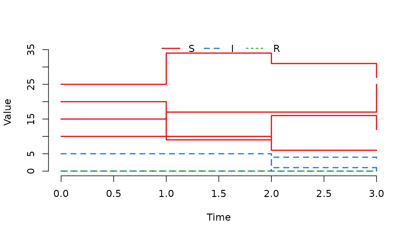

Figure 2. Number of susceptible, infected and recovered individuals in each node.

$~$

Or use the trajectory() function to more easily inspect the outcome in each node in detail.

trajectory(result)

##    node time  S I R
## 1     1    0 10 5 0
## 2     2    0 15 0 0
## 3     3    0 20 0 0
## 4     4    0 25 0 0
## 5     1    1 10 5 0
## 6     2    1 17 0 0
## 7     3    1  9 0 0
## 8     4    1 34 0 0
## 9     1    2  6 1 0
## 10    2    2 17 0 0
## 11    3    2 16 4 0
## 12    4    2 31 0 0
## 13    1    3  6 1 0
## 14    2    3 25 1 0
## 15    3    3 12 3 0
## 16    4    3 27 0 0

Varying probability of picking individuals

It is possible to assign different probabillities for the compartments that an event sample individuals from. If the weights in the select matrix $E$ are non-identical, individuals are sampled from a biased urn. To illustrate this, let us create movement events between two nodes for the built-in SIR model, where we start with 300 individuals ( $S = 100$ , $I = 100$ , $R = 100$ ) in the first node and then move them, one by one, to the second node.

u0 <- data.frame(S = c(100, 0),
                 I = c(100, 0),
                 R = c(100, 0))

events <- data.frame(
  event = rep("extTrans", 300), ## Event "extTrans" is a movement between nodes
  time = 1:300,                 ## The time that the event happens
  node = 1,                     ## In which node does the event occur
  dest = 2,                     ## Which node is the destination node
  n = 1,                        ## How many individuals are moved
  proportion = 0,               ## This is not used when n > 0
  select = 4,                   ## Use the 4th column in the model select matrix
  shift = 0)                    ## Not used in this example

Now, create the model. Then run it, and plot the number of individuals in the second node.

model <- SIR(u0 = u0,
             tspan = 1:300,
             events = events,
             beta = 0,
             gamma = 0)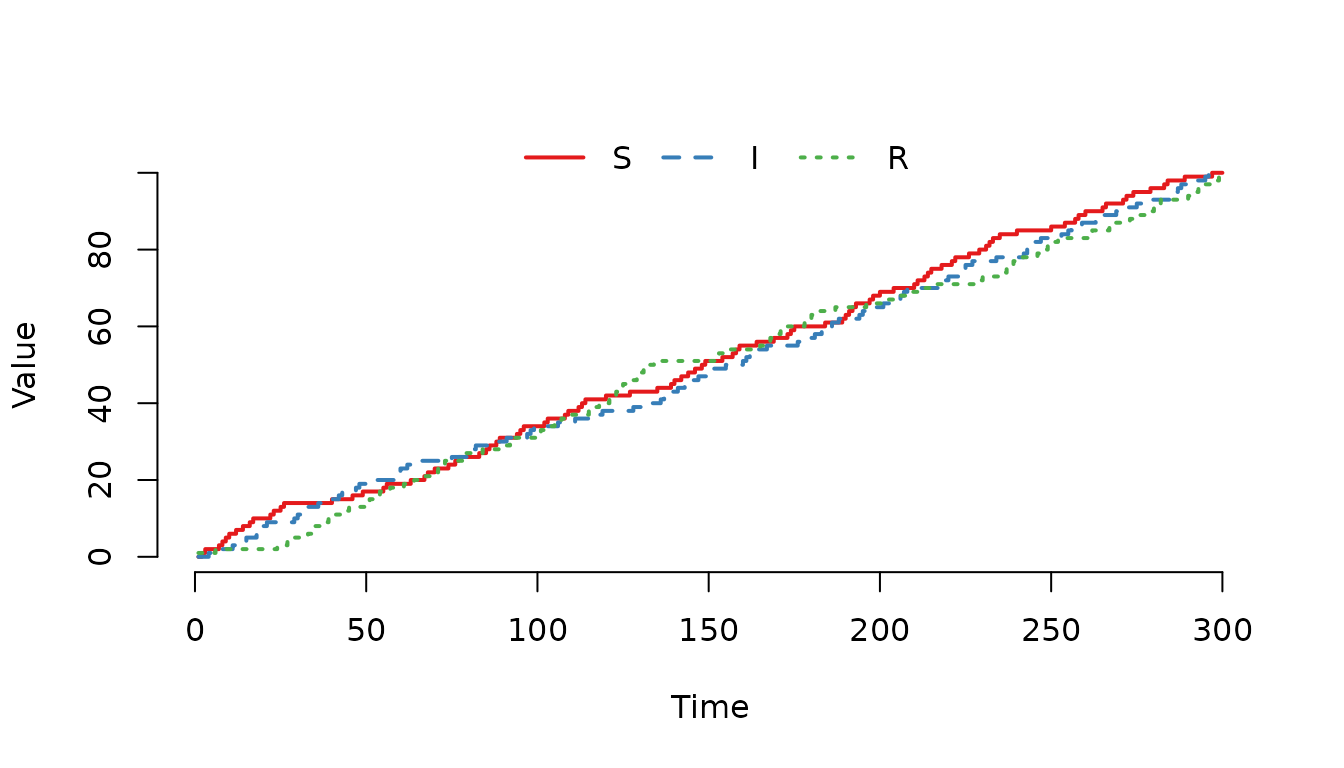

plot(run(model), index = 2)

Figure 3. The individuals have an equal probability of being selected regardless of compartment.

$~$

The probability to sample an individual from each compartment is

$p_S = \frac{w_S * S}{w_S * S + w_I * I + w_R * R}$

$p_I = \frac{w_I * I}{w_S * S + w_I * I + w_R * R}$

$p_R = \frac{w_R * R}{w_S * S + w_I * I + w_R * R}$

Where $w_S$ , $w_I$ and $w_R$ are the weights in E. These probabilities are applied sequentially, that is the probability of choosing the next item is proportional to the weights amongst the remaining items. Let us now double the weight to sample individuals from the $I$ compartment and then run the model again.

model@events@E[2, 4] <- 2
plot(run(model), index = 2)

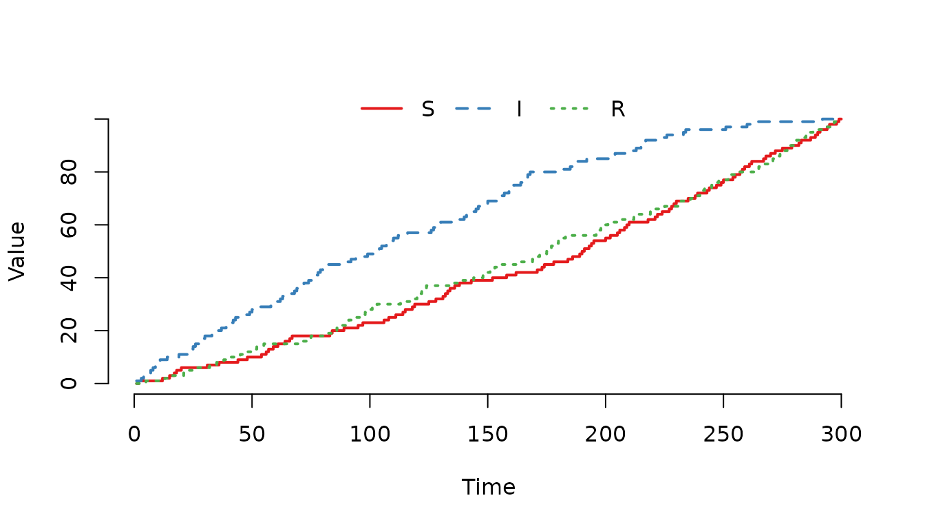
Figure 4. The individuals in the $I$ compartment are more likely of being selected for a movement event.

$~$

And a much larger weight to sample individuals from the $I$ compartment.

model@events@E[2, 4] <- 10
plot(run(model), index = 2)

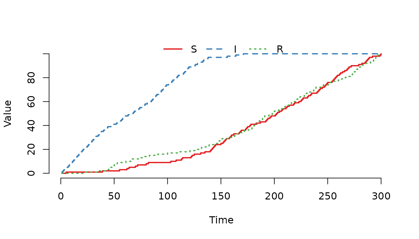
Figure 5. The individuals in the $I$ compartment are even more likely of being selected for a movement event compared to the previous example.

$~$

Increase the weight for the $R$ compartment and run the model again.

model@events@E[3, 4] <- 4
plot(run(model), index = 2)

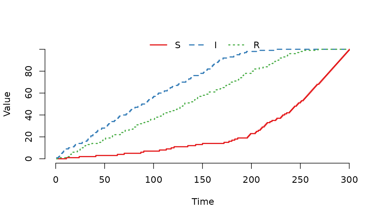
Figure 6. The individuals in the $I$ and $R$ compartments are more likely of being selected for a movement event compared to individuals in the $S$ compartment.

Enter events: Adding individuals

Enter events are used to add individuals to a node. A common use case is modelling births in a population. New individuals can be added to specific compartments, and the E matrix weights determine which compartments receive the new individuals when multiple compartments are selected.

Example: Births entering a population

Let us create a simple model where births occur at regular intervals. Newborns enter the susceptible compartment.

u0 <- data.frame(S = 20, I = 10, R = 0)

We schedule births at times 5, 10, and 15, adding 10 individuals each time. All newborns enter the susceptible compartment (column 1 in the E matrix).

events <- data.frame(
  event      = rep("enter", 3), ## "enter" add new individuals to a node
  time       = c(5, 10, 15),    ## The time that the event happens
  node       = c(1, 1, 1),      ## In which node does the event occur
  dest       = c(0, 0, 0),      ## Not used for enter events
  n          = c(10, 10, 10),   ## How many individuals are added
  proportion = c(0, 0, 0),      ## Not used when n > 0
  select     = c(1, 1, 1),      ## Target the S compartment
  shift      = c(0, 0, 0))      ## Not used in this example

model <- SIR(u0 = u0,
             tspan = 0:20,
             events = events,
             beta = 0,
             gamma = 0)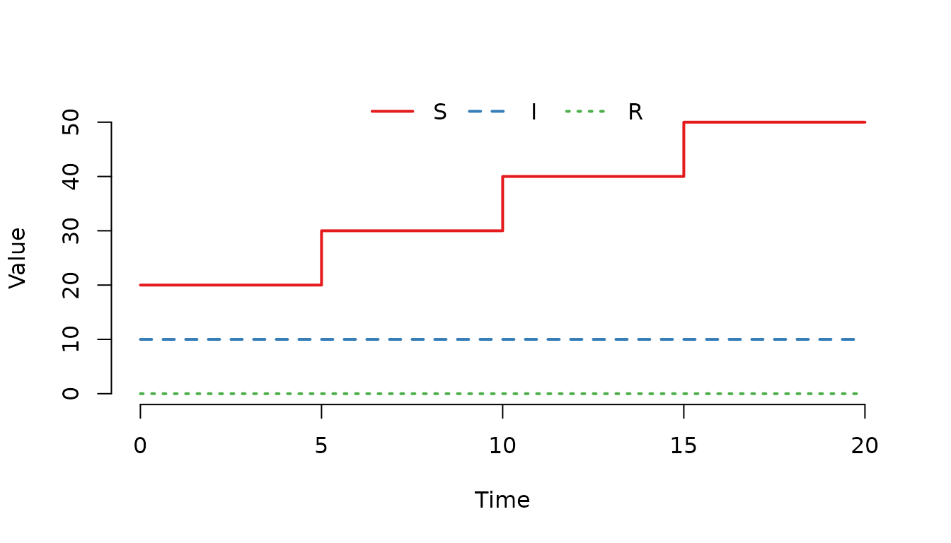

plot(run(model))

Figure 7. The number of susceptible ( $S$ ) individuals increases by 10 individuals at each scheduled event.

Weighted sampling for enter events

When the $E[, select]$ column contains multiple non-zero entries, the new individuals are distributed among the compartments with probability proportional to the weights. Let us demonstrate this by creating a scenario where newborns can enter either $S$ or $R$ compartments. First, create the initial state and the scheduled events. We will use select=1 and show how we can adjust the select matrix to include both the $S$ and $R$ compartments for that select value.

u0 <- data.frame(S = 20, I = 10, R = 0)

We schedule one birth event per day for 300 days, adding 1 individual each time. We want each newborn to enter either the susceptible or the recovered compartment, with probability proportional to the weights in column 1 of the E matrix.

events <- data.frame(
  event      = rep("enter", 300), ## "enter" add new individuals to a node
  time       = 1:300,             ## The time that the event happens
  node       = rep(1, 300),       ## In which node does the event occur
  dest       = rep(0, 300),       ## Not used for enter events
  n          = rep(1, 300),       ## How many individuals are added
  proportion = rep(0, 300),       ## Not used when n > 0
  select     = rep(1, 300),       ## Target the S and R compartments
                                  ## (after modifying E)
  shift      = rep(0, 300))       ## Not used in this example

model <- SIR(u0 = u0,
             tspan = 0:300,
             events = events,
             beta = 0,
             gamma = 0)

Let us now change the select matrix so that we can use our events as expected. It is not necessary to use value=1 since that is the default, however, for clarity we specifically set that value.

select_matrix(model) <- data.frame(
  compartment = c("S", "R"),
  select      = c(1, 1),
  value       = c(1, 1))

Now, verify the select matrix.

select_matrix(model)

## 3 x 1 sparse Matrix of class "dgCMatrix"
##   1
## S 1
## I .
## R 1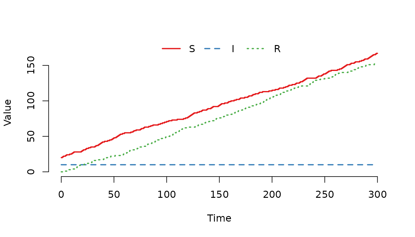

plot(run(model))

Figure 8. The number of susceptible ( $S$ ) and recovered ($R) individuals increases over time.

Let us modify the E matrix so that newborns are more likely to enter the S compartment compared to the R compartment.

select_matrix(model) <- data.frame(
  compartment = c("S", "R"),
  select      = c(1, 1),
  value       = c(2, 1))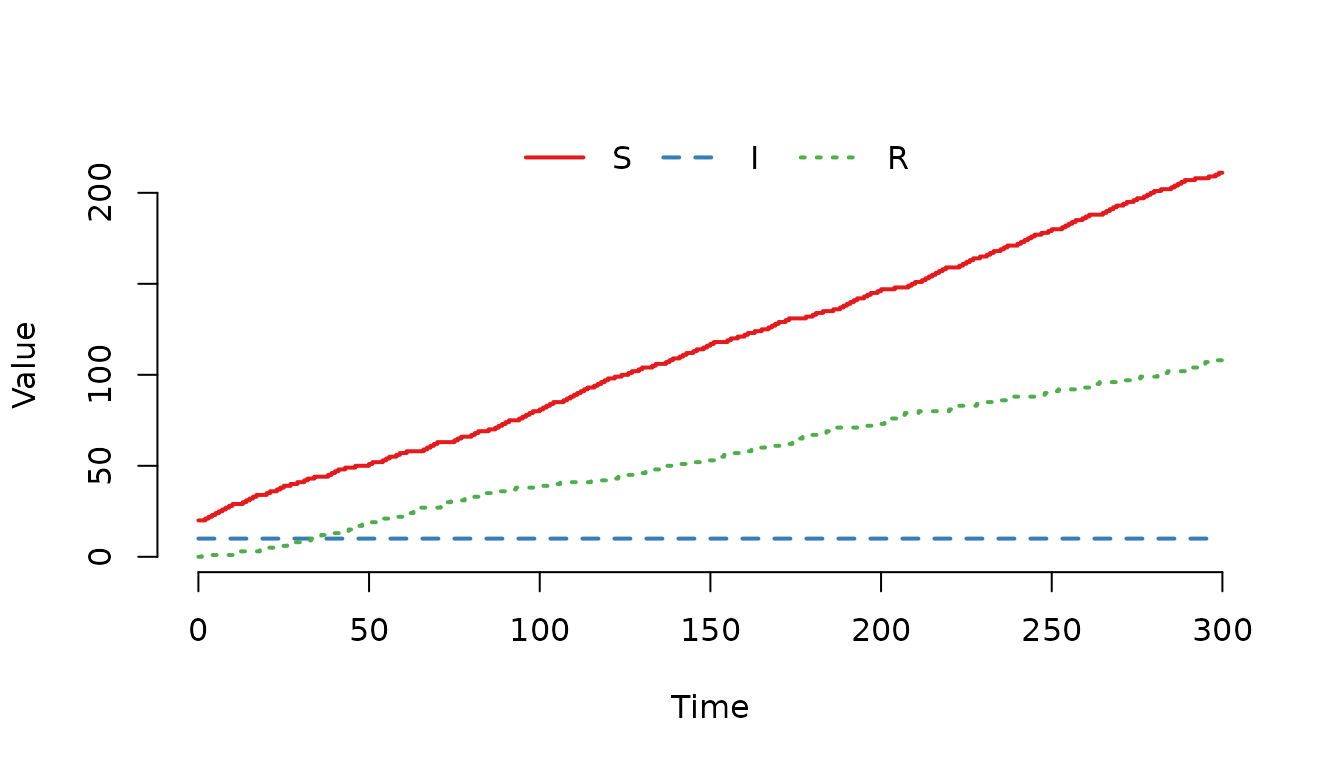

plot(run(model))

Figure 9. Individuals are more likely to enter as susceptible ( $S$ ) compared to as recovered ( $R$ )

Exit events: Removing individuals

Exit events remove individuals from a node. Common use cases include natural mortality or culling. Like enter events, the E matrix weights determine which compartments individuals are removed from when multiple compartments are selected.

Example: Mortality

Let us create a model where individuals die at scheduled times.

u0 <- data.frame(S = 20, I = 10, R = 0)

events <- data.frame(
  event      = rep("exit", 3),  ## "exit" remove individuals from a node
  time       = c(5, 10, 15),    ## The time that the event happens
  node       = c(1, 1, 1),      ## In which node does the event occur
  dest       = c(0, 0, 0),      ## Not used for exit events
  n          = c(5, 5, 5),      ## How many individuals are removed
  proportion = c(0, 0, 0),      ## Not used when n > 0
  select     = c(1, 1, 1),      ## Target the S compartment
  shift      = c(0, 0, 0))      ## Not used in this example

model <- SIR(u0 = u0,
             tspan = 0:20,
             events = events,
             beta = 0,
             gamma = 0)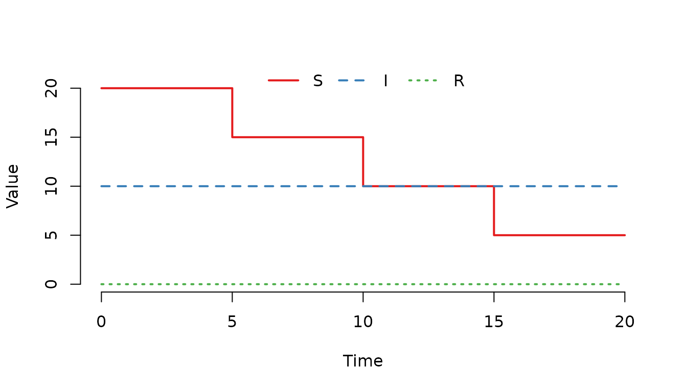

plot(run(model))

Figure 10. The number of susceptible ( $S$ ) individuals decreases by 5 individuals at each scheduled event.

Weighted sampling for exit events

We can also use weights to make certain compartments more likely to lose individuals. For example, infected individuals might have higher mortality risk.

u0 <- data.frame(S = 100, I = 100, R = 0)

events <- data.frame(
  event      = rep("exit", 100), ## "exit" remove individuals from a node
  time       = 1:100,            ## The time that the event happens
  node       = rep(1, 100),      ## In which node does the event occur
  dest       = rep(0, 100),      ## Not used for exit events
  n          = rep(1, 100),      ## How many individuals are removed
  proportion = rep(0, 100),      ## Not used when n > 0
  select     = rep(1, 100),      ## Target the S and I compartments
                                 ## (after modifying E)
  shift      = rep(0, 100))      ## Not used in this example

model <- SIR(u0 = u0,
             tspan = 0:100,
             events = events,
             beta = 0,
             gamma = 0)

Let us increase the weight for the I compartment to make infected individuals more likely to be removed:

select_matrix(model) <- data.frame(
  compartment = c("S", "I"),
  select      = c(1, 1),
  value       = c(1, 5))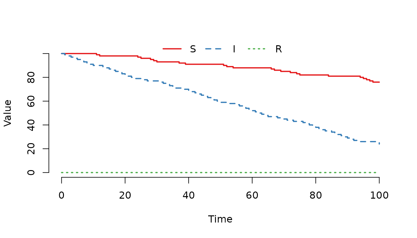

plot(run(model))

Figure 11. The number of infected ( $I$ ) individuals decreases faster compared to susceptibles ( $S$ ).

Internal transfer events: Moving within a node

Internal transfer events move individuals between compartments within the same node. Common use cases include vaccination (moving from S to R or V), ageing between age-structured compartments, or treatment effects.

Example: Vaccination of cattle herd

Let us create a model where a vaccination campaign moves susceptible individuals to the recovered compartment at a specific time. We will use shift=1 and show how we can adjust the shift matrix to move susceptible to recovered.

u0 <- data.frame(S = 100, I = 10, R = 0)

At time 10, we vaccinate 30 susceptible individuals, moving them to the R compartment.

events <- data.frame(
  event      = "intTrans", ## "intTrans" move individuals within a node
  time       = 10,         ## The time that the event happens
  node       = 1,          ## In which node does the event occur
  dest       = 0,          ## Not used for intTrans events
  n          = 30,         ## How many individuals are vaccinated
  proportion = 0,          ## Not used when n > 0
  select     = 1,          ## Target the S compartment
  shift      = 1)          ## Use shift column 1 (after modifying N)

model <- SIR(u0 = u0,
             tspan = 0:20,
             events = events,
             beta = 0,
             gamma = 0)

Let us now change the shift matrix so that we can use our events as expected. Susceptible individuals will be moved to the recovered compartment. With compartments ordered S=1, I=2, R=3, a value of 2 means individuals from compartment 1 (S) move to compartment 1+2=3 (R).

shift_matrix(model) <- data.frame(compartment = "S", shift = 1, value = 2)

Note: Unlike the select_matrix() function where the value column is optional (defaulting to 1), the value column is mandatory when using a data.frame with shift_matrix(). This is because the N matrix stores integer offsets (how many rows to shift) rather than just presence/absence indicators, so the specific shift amount must be explicitly defined. The shift parameter works together with the shift matrix (N) to determine the destination compartment.

Now, verify the shift matrix.

shift_matrix(model)

##   1
## S 2
## I 0
## R 0

Each column in N defines a different transfer pattern. The shift value selects which column to use. The value N[p, q] indicates how many rows to move from compartment p.

plot(run(model))

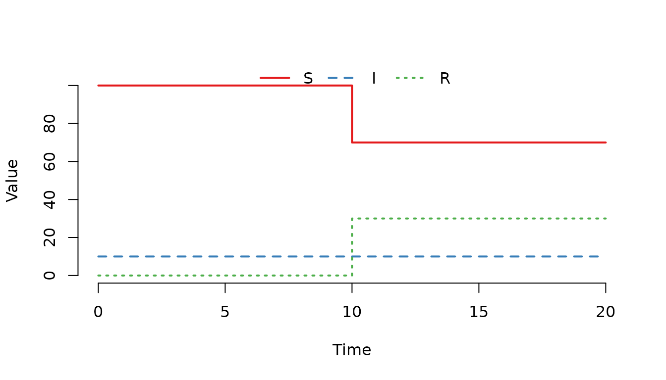
Figure 12. The number of recovered ( $R$ ) individuals increases at $t=10$ .

Stochastic events using proportion

Instead of specifying a fixed number n, events can use proportion to sample a proportion of individuals from the selected compartments. This is useful when you want to remove or move a percentage of the population.

Example: Proportional culling

u0 <- data.frame(S = 20, I = 15, R = 10)

Remove 20% of the population at time 10:

events <- data.frame(
  event      = "exit", ## "exit" remove individuals from a node
  time       = 10,     ## The time that the event happens
  node       = 1,      ## In which node does the event occur
  dest       = 0,      ## Not used for exit events
  n          = 0,      ## n = 0 triggers proportion sampling
  proportion = 0.2,    ## Remove 20% of selected individuals
  select     = 4,      ## Target all compartments
  shift      = 0)      ## Not used in this example

model <- SIR(u0 = u0,
             tspan = 0:20,
             events = events,
             beta = 0,
             gamma = 0)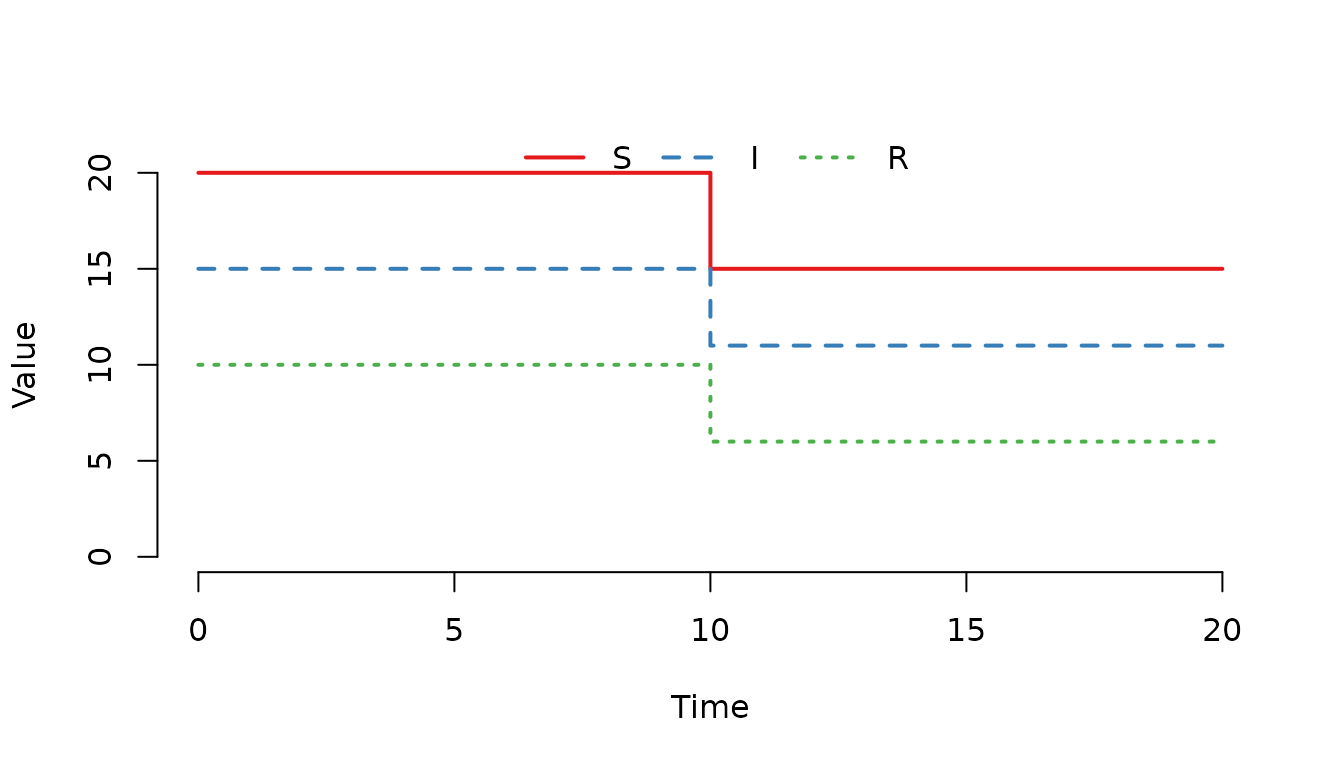

plot(run(model))

Figure 13. The number of individuals decrease at $t=10$ .

Processing order of simultaneous events

When multiple events are scheduled at the same time point, they are processed in a specific order:

Exit events (removals)
Enter events (additions)
Internal transfer events (within-node movements)
External transfer events (between-node movements)

This ordering ensures that removals happen before additions, and within-node movements happen before between-node movements.

Example: Multiple events at the same time

u0 <- data.frame(
  S = c(20, 30),
  I = c(15, 25),
  R = c(10, 5))

At time 5, we schedule:

10 deaths (exit)
20 births (enter)
5 vaccinations (internal transfer)
15 movements to node 2 (external transfer)

events <- data.frame(
  event      = c("exit", "enter", "intTrans", "extTrans"),
  time       = c(5, 5, 5, 5),
  node       = c(1, 1, 1, 1),
  dest       = c(0, 0, 0, 2),
  n          = c(10, 20, 5, 15),
  proportion = c(0, 0, 0, 0),
  select     = c(4, 1, 1, 4),
  shift      = c(0, 0, 1, 0))

model <- SIR(u0 = u0,
             tspan = 0:10,
             events = events,
             beta = 0,
             gamma = 0)

shift_matrix(model) <- data.frame(compartment = "S", shift = 1, value = 2)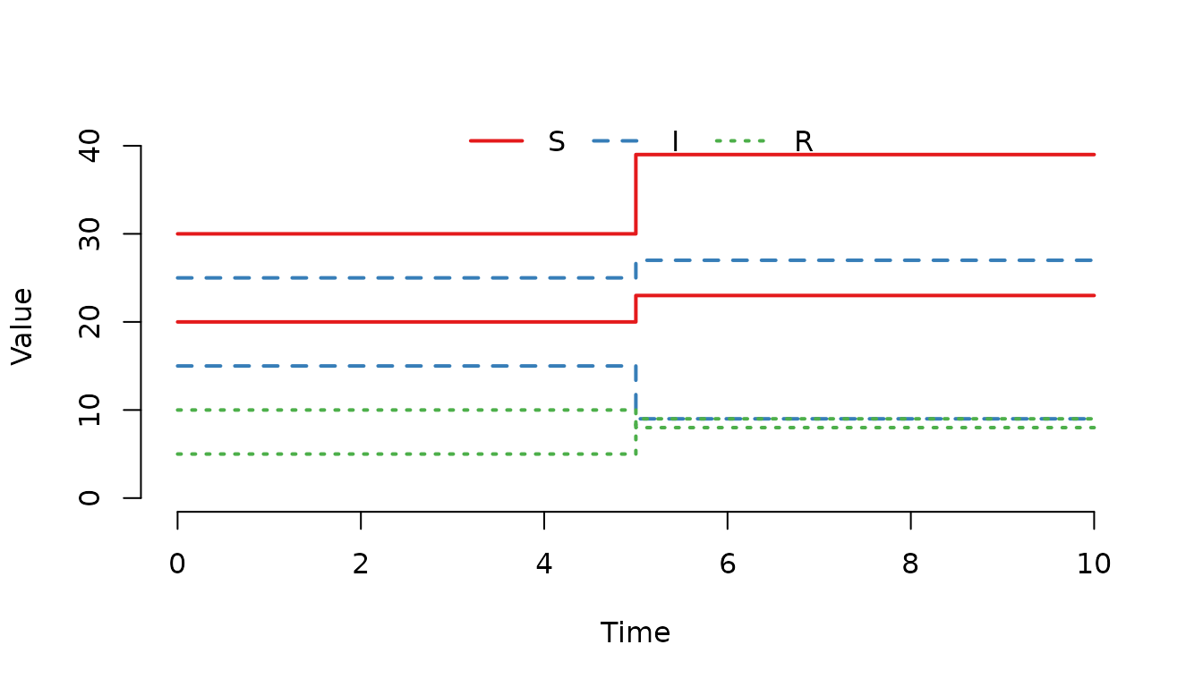

plot(run(model), range = FALSE)

Figure 14. Multiple events have been processed at $t=5$ .

Summary

This vignette demonstrated the four types of scheduled events in SimInf:

Event type	Purpose	Key parameters
`enter`	Add individuals to a node	`n` or `proportion`, `select`, `shift`
`exit`	Remove individuals from a node	`n` or `proportion`, `select`
`intTrans`	Move individuals within a node	`n` or `proportion`, `select`, `shift`
`extTrans`	Move individuals between nodes	`n` or `proportion`, `select`, `shift`, `dest`

Key points to remember:

The E matrix determines which compartments are affected by each event type via the select parameter
Values in the E matrix are used as weights for sampling individuals when multiple compartments are selected
Events at the same time are processed in the order: exit, enter, internal transfer, external transfer
Use n for deterministic numbers or proportion for stochastic sampling

For more detailed information about the SimInf_events class and the underlying algorithms, see the package documentation and the accompanying technical paper.

Stefan Widgren