Dataset containing the initial number of susceptible, infected, and recovered cattle across 1,600 herds. Provides realistic population structure for demonstrating SIR model simulations in a cattle disease epidemiology context.
Value
A data.frame with 1,600 rows (one per herd) and 3 columns:
- S
Number of susceptible cattle in the herd
- I
Number of infected cattle in the herd (all zero at start)
- R
Number of recovered cattle in the herd (all zero at start)
Details
This dataset represents initial disease states in a population of
1,600 cattle herds. Each node (row) represents a single herd, and
the data is derived from the structured u0_SISe3 data by
aggregating age-stratified compartments into single S, I, and R
compartments for each herd.
The aggregated values represent:
- S
Total susceptible cattle across all age groups in the herd
- I
Total infected cattle (initialized to zero)
- R
Total recovered cattle (initialized to zero)
The herd size distribution reflects realistic heterogeneity observed in cattle populations, making it suitable for testing spatial disease dynamics at the herd level, such as:
Transmission within and between herds
Impact of cattle movement on disease spread
Effectiveness of herd-level interventions
See also
SIR for creating cattle disease models with this
initial state and events_SIR for associated cattle
movement and demographic events
Examples
## For reproducibility, call the set.seed() function and specify the
## number of threads to use. To use all available threads, remove the
## set_num_threads() call.
set.seed(123)
set_num_threads(1)
## Create an 'SIR' model with 1600 cattle herds (nodes) and initialize
## it to run over 4*365 days. Add one infected animal to the first
## herd to seed the outbreak. Define 'tspan' to record the state of
## the system at daily time-points. Load scheduled events for the
## population of nodes with births, deaths and between-node movements
## of individuals.
u0 <- u0_SIR()
u0$I[1] <- 1
model <- SIR(u0 = u0,
tspan = seq(from = 1, to = 4*365, by = 1),
events = events_SIR(),
beta = 0.16,
gamma = 0.01)
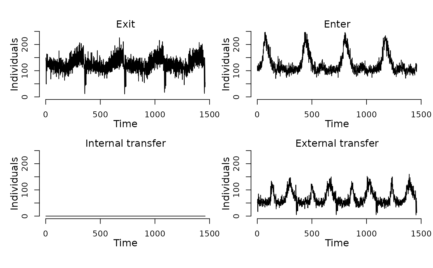
## Display the number of cattle affected by each event type per day.
plot(events(model))
 ## Run the model to generate a single stochastic trajectory.
result <- run(model)
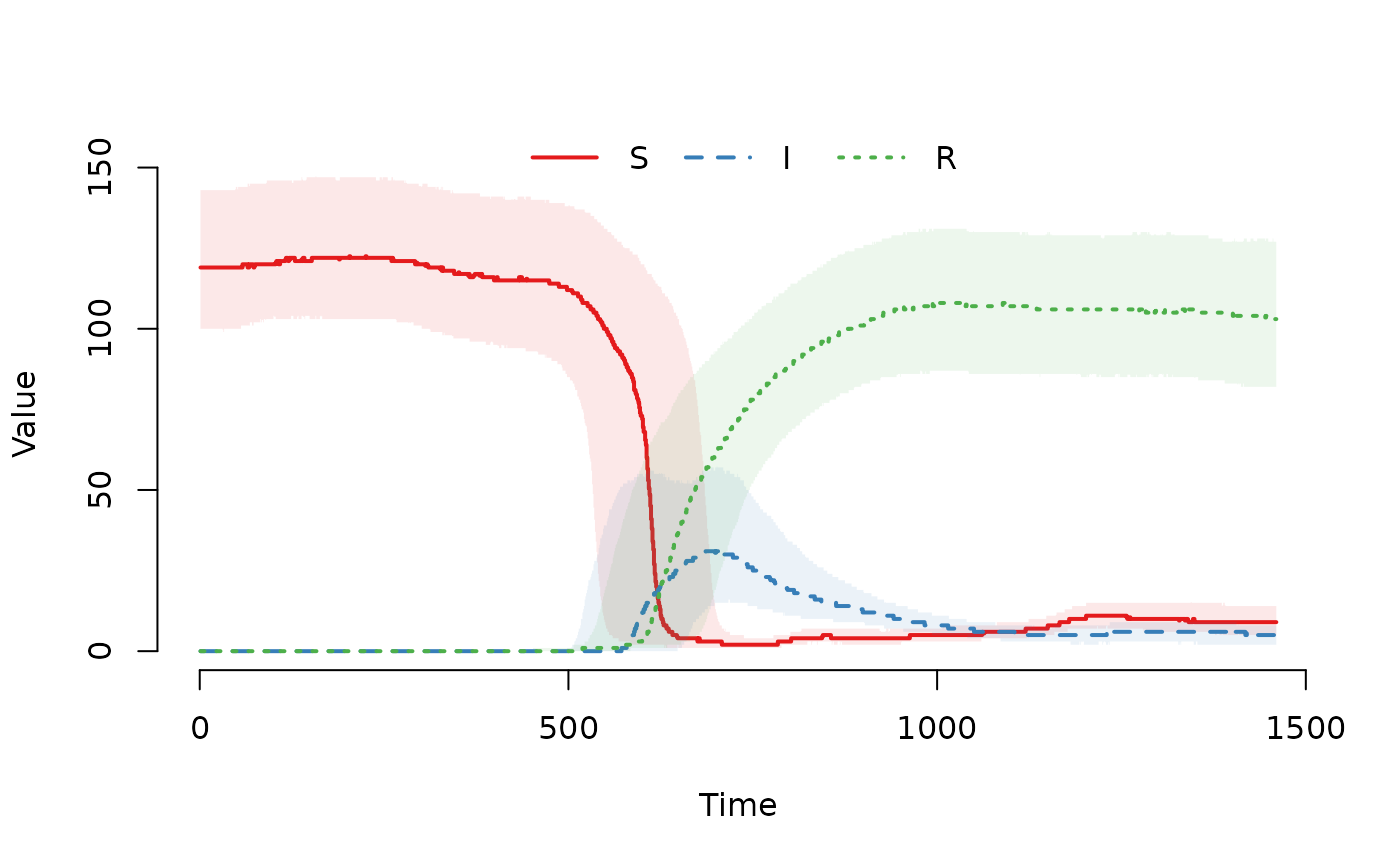
## Plot the median and interquartile range of the number of
## susceptible, infected and recovered individuals.
plot(result)
## Run the model to generate a single stochastic trajectory.
result <- run(model)
## Plot the median and interquartile range of the number of
## susceptible, infected and recovered individuals.
plot(result)
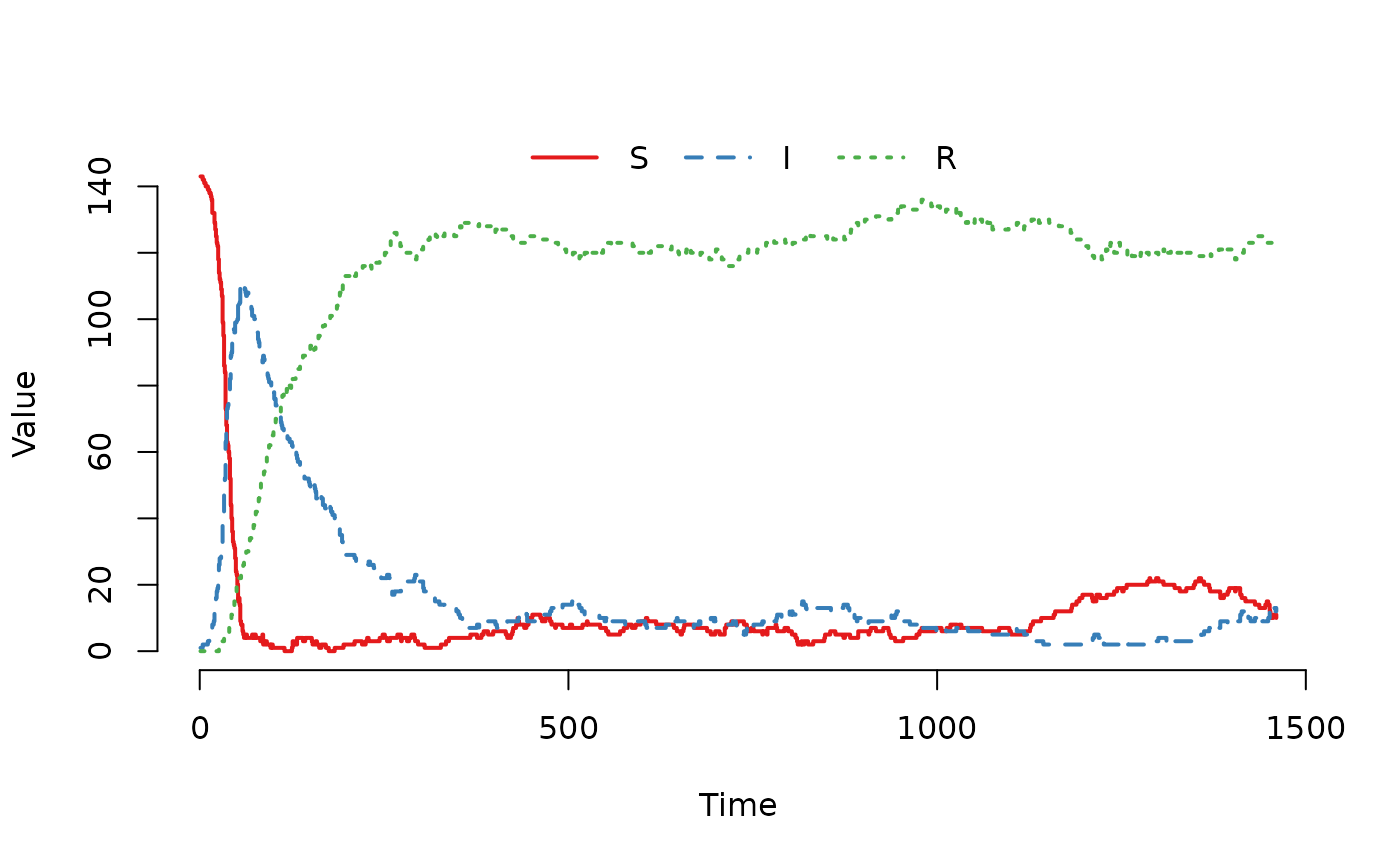
 ## Plot the trajectory for the first herd.
plot(result, index = 1)
## Plot the trajectory for the first herd.
plot(result, index = 1)
 ## Summarize the trajectory. The summary includes the number of events
## by event type.
summary(result)
#> Model: SIR
#> Number of nodes: 1600
#>
#> Transitions
#> -----------
#> S -> beta*S*I/(S+I+R) -> I
#> I -> gamma*I -> R
#>
#> Global data
#> -----------
#> Number of parameters without a name: 0
#> - None
#>
#> Local data
#> ----------
#> Parameter Value
#> beta 0.16
#> gamma 0.01
#>
#> Scheduled events
#> ----------------
#> Exit: 182535
#> Enter: 182685
#> Internal transfer: 0
#> External transfer: 101472
#>
#> Network summary
#> ---------------
#> Min. 1st Qu. Median Mean 3rd Qu. Max.
#> Indegree: 40.0 57.0 62.0 62.1 68.0 90.0
#> Outdegree: 36.0 57.0 62.0 62.1 67.0 89.0
#>
#> Compartments
#> ------------
#> Min. 1st Qu. Median Mean 3rd Qu. Max.
#> S 0.0 5.0 13.0 55.6 112.0 219.0
#> I 0.0 0.0 4.0 10.9 11.0 168.0
#> R 0.0 0.0 62.0 58.0 105.0 221.0
## Summarize the trajectory. The summary includes the number of events
## by event type.
summary(result)
#> Model: SIR
#> Number of nodes: 1600
#>
#> Transitions
#> -----------
#> S -> beta*S*I/(S+I+R) -> I
#> I -> gamma*I -> R
#>
#> Global data
#> -----------
#> Number of parameters without a name: 0
#> - None
#>
#> Local data
#> ----------
#> Parameter Value
#> beta 0.16
#> gamma 0.01
#>
#> Scheduled events
#> ----------------
#> Exit: 182535
#> Enter: 182685
#> Internal transfer: 0
#> External transfer: 101472
#>
#> Network summary
#> ---------------
#> Min. 1st Qu. Median Mean 3rd Qu. Max.
#> Indegree: 40.0 57.0 62.0 62.1 68.0 90.0
#> Outdegree: 36.0 57.0 62.0 62.1 67.0 89.0
#>
#> Compartments
#> ------------
#> Min. 1st Qu. Median Mean 3rd Qu. Max.
#> S 0.0 5.0 13.0 55.6 112.0 219.0
#> I 0.0 0.0 4.0 10.9 11.0 168.0
#> R 0.0 0.0 62.0 58.0 105.0 221.0