Dataset containing 466,692 scheduled events for a population of 1,600 cattle herds over 1,460 days (4 years). Demonstrates how demographic and movement events affect SISe dynamics in a cattle disease context.
Value
A data.frame with columns:
- event
Event type: "exit", "enter", or "extTrans".
- time
Day when event occurs (1-1460).
- node
Affected herd identifier (1-1600).
- dest
Destination herd for external transfer events.
- n
Number of cattle affected.
- proportion
0. Not used in this example.
- select
Model compartment to affect (see
SimInf_events).- shift
0. Not used in this example.
Details
The event data contains three types of scheduled events that affect cattle herds:
- Exit
Deaths or removal of cattle from a herd (n = 182,535). These events decrease the population in susceptible and infected compartments.
- Enter
Births or introduction of cattle to a herd (n = 182,685). These events add susceptible cattle to herds.
- External transfer
Movement of cattle between herds (n = 101,472). These events transfer cattle from one herd to another, potentially introducing infected animals.
The select column in the returned data frame is mapped to
the columns of the internal select matrix (select_matrix_SISe):
select = 1corresponds to Enter events, targeting the Susceptible (S) compartment.select = 2corresponds to Exit and External Transfer events, targeting all compartments (S and I).
Events are distributed across all 1,600 herds over the 4-year period. These are synthetic data generated to illustrate how to incorporate scheduled events (such as births, deaths, and movements) into a compartment model in the SimInf framework.
See also
u0_SISe for the corresponding initial cattle
population, SISe for creating SISe models with these
events and SimInf_events for event structure
details
Examples
## For reproducibility, call the set.seed() function and specify the
## number of threads to use. To use all available threads, remove the
## set_num_threads() call.
set.seed(123)
set_num_threads(1)
## Create an 'SISe' model with 1600 cattle herds (nodes) and
## initialize it to run over 4*365 days. Add ten infected animals to
## the first herd. Define 'tspan' to record the state of the system at
## weekly time-points. Load scheduled events for the population of
## nodes with births, deaths and between-node movements of
## individuals.
u0 <- u0_SISe()
u0$I[1] <- 10
model <- SISe(
u0 = u0,
tspan = seq(from = 1, to = 4*365, by = 7),
events = events_SISe(),
phi = 0,
upsilon = 1.8e-2,
gamma = 0.1,
alpha = 1,
beta_t1 = 1.0e-1,
beta_t2 = 1.0e-1,
beta_t3 = 1.25e-1,
beta_t4 = 1.25e-1,
end_t1 = 91,
end_t2 = 182,
end_t3 = 273,
end_t4 = 365,
epsilon = 0
)
## Display the number of cattle affected by each event type per day.
plot(events(model))
 ## Run the model to generate a single stochastic trajectory.
result <- run(model)
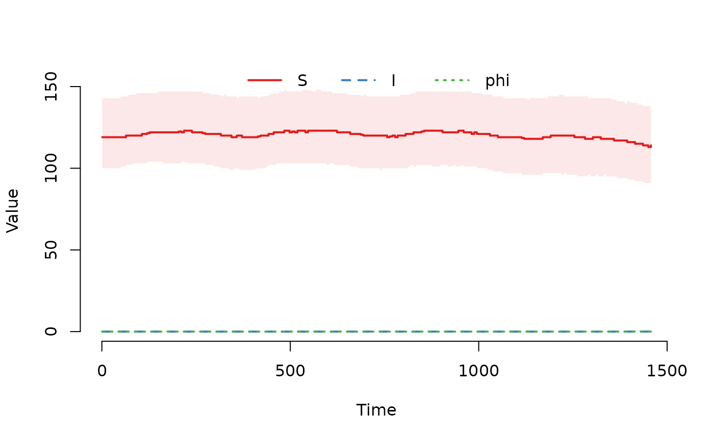
## Plot the median and interquartile range of the number of
## susceptible and infected individuals.
plot(result)
## Run the model to generate a single stochastic trajectory.
result <- run(model)
## Plot the median and interquartile range of the number of
## susceptible and infected individuals.
plot(result)
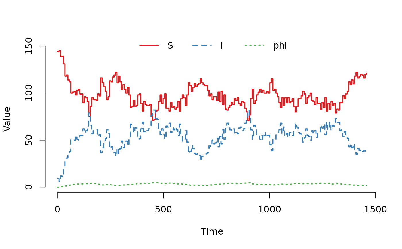
 ## Plot the trajectory for the first herd.
plot(result, index = 1)
## Plot the trajectory for the first herd.
plot(result, index = 1)
 ## Summarize the trajectory. The summary includes the number of events
## by event type.
summary(result)
#> Model: SISe
#> Number of nodes: 1600
#>
#> Transitions
#> -----------
#> S -> upsilon*phi*S -> I
#> I -> gamma*I -> S
#>
#> Global data
#> -----------
#> Parameter Value
#> upsilon 0.018
#> gamma 0.100
#> alpha 1.000
#> beta_t1 0.100
#> beta_t2 0.100
#> beta_t3 0.125
#> beta_t4 0.125
#> epsilon 0.000
#>
#> Local data
#> ----------
#> Parameter Value
#> end_t1 91
#> end_t2 182
#> end_t3 273
#> end_t4 365
#>
#> Scheduled events
#> ----------------
#> Exit: 182535
#> Enter: 182685
#> Internal transfer: 0
#> External transfer: 101472
#>
#> Network summary
#> ---------------
#> Min. 1st Qu. Median Mean 3rd Qu. Max.
#> Indegree: 40.0 57.0 62.0 62.1 68.0 90.0
#> Outdegree: 36.0 57.0 62.0 62.1 67.0 89.0
#>
#> Continuous state variables
#> --------------------------
#> Min. 1st Qu. Median Mean 3rd Qu. Max.
#> phi 0.000 0.000 0.000 0.108 0.000 5.548
#>
#> Compartments
#> ------------
#> Min. 1st Qu. Median Mean 3rd Qu. Max.
#> S 18.00 100.00 120.00 122.97 145.00 237.00
#> I 0.00 0.00 0.00 1.57 0.00 100.00
## Summarize the trajectory. The summary includes the number of events
## by event type.
summary(result)
#> Model: SISe
#> Number of nodes: 1600
#>
#> Transitions
#> -----------
#> S -> upsilon*phi*S -> I
#> I -> gamma*I -> S
#>
#> Global data
#> -----------
#> Parameter Value
#> upsilon 0.018
#> gamma 0.100
#> alpha 1.000
#> beta_t1 0.100
#> beta_t2 0.100
#> beta_t3 0.125
#> beta_t4 0.125
#> epsilon 0.000
#>
#> Local data
#> ----------
#> Parameter Value
#> end_t1 91
#> end_t2 182
#> end_t3 273
#> end_t4 365
#>
#> Scheduled events
#> ----------------
#> Exit: 182535
#> Enter: 182685
#> Internal transfer: 0
#> External transfer: 101472
#>
#> Network summary
#> ---------------
#> Min. 1st Qu. Median Mean 3rd Qu. Max.
#> Indegree: 40.0 57.0 62.0 62.1 68.0 90.0
#> Outdegree: 36.0 57.0 62.0 62.1 67.0 89.0
#>
#> Continuous state variables
#> --------------------------
#> Min. 1st Qu. Median Mean 3rd Qu. Max.
#> phi 0.000 0.000 0.000 0.108 0.000 5.548
#>
#> Compartments
#> ------------
#> Min. 1st Qu. Median Mean 3rd Qu. Max.
#> S 18.00 100.00 120.00 122.97 145.00 237.00
#> I 0.00 0.00 0.00 1.57 0.00 100.00