Dataset containing the initial number of susceptible, exposed, infected, and recovered cattle across 1,600 herds. Provides realistic population structure for demonstrating SEIR model simulations in a cattle disease epidemiology context.
Value
A data.frame with 1,600 rows (one per herd) and 4 columns:
- S
Number of susceptible cattle in the herd
- E
Number of exposed cattle in the herd (all zero at start)
- I
Number of infected cattle in the herd (all zero at start)
- R
Number of recovered cattle in the herd (all zero at start)
Details
This dataset represents initial disease states in a population of 1,600 cattle herds (nodes). Each row represents a single herd (node), derived from the structured cattle population data by adding an exposed compartment to the SIR model structure.
The data contains:
- S
Total susceptible cattle in the herd
- E
Total exposed cattle (initialized to zero)
- I
Total infected cattle (initialized to zero)
- R
Total recovered cattle (initialized to zero)
The herd size distribution reflects realistic heterogeneity observed in cattle populations, making it suitable for testing disease dynamics with an explicit latent period.
See also
SEIR for creating SEIR models with this initial
state and events_SEIR for associated cattle movement
and demographic events
Examples
## For reproducibility, call the set.seed() function and specify the
## number of threads to use. To use all available threads, remove the
## set_num_threads() call.
set.seed(123)
set_num_threads(1)
## Create a 'SEIR' model with 1600 cattle herds (nodes) and initialize
## it to run over 4*365 days. Add ten exposed animals to the first
## herd. Define 'tspan' to record the state of the system at weekly
## time-points. Load scheduled events for the population of nodes with
## births, deaths and between-node movements of individuals.
u0 <- u0_SEIR()
u0$E[1] <- 10
model <- SEIR(u0 = u0,
tspan = seq(from = 1, to = 4*365, by = 7),
events = events_SEIR(),
beta = 0.16,
epsilon = 0.25,
gamma = 0.01)
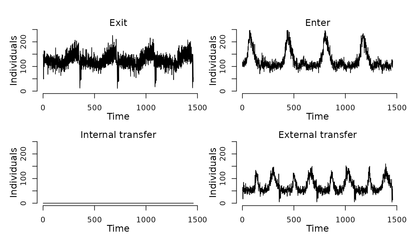
## Display the number of cattle affected by each event type per day.
plot(events(model))
 ## Run the model to generate a single stochastic trajectory.
result <- run(model)
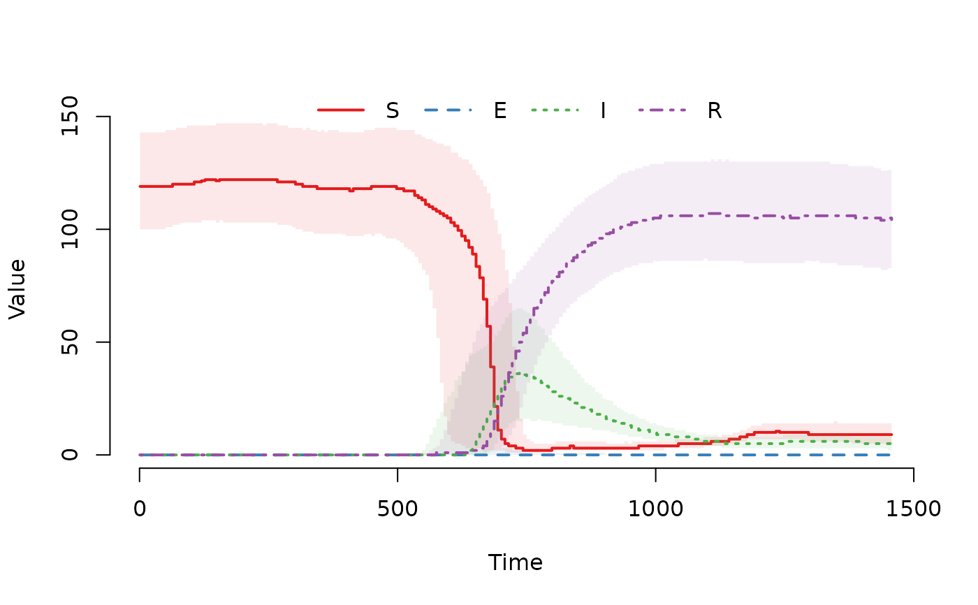
## Plot the median and interquartile range of the number of
## susceptible, exposed, infected and recovered individuals.
plot(result)
## Run the model to generate a single stochastic trajectory.
result <- run(model)
## Plot the median and interquartile range of the number of
## susceptible, exposed, infected and recovered individuals.
plot(result)
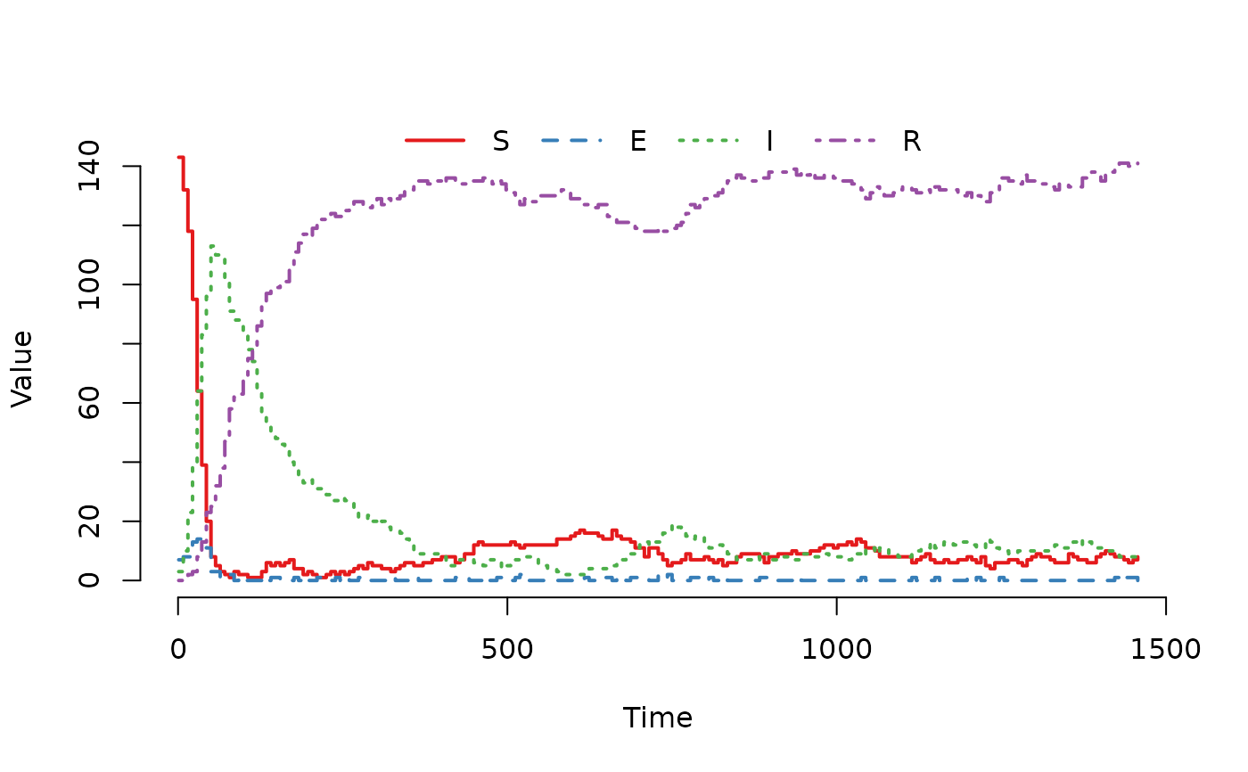
 ## Plot the trajectory for the first herd.
plot(result, index = 1)
## Plot the trajectory for the first herd.
plot(result, index = 1)
 ## Summarize the trajectory. The summary includes the number of events
## by event type.
summary(result)
#> Model: SEIR
#> Number of nodes: 1600
#>
#> Transitions
#> -----------
#> S -> beta*S*I/(S+E+I+R) -> E
#> E -> epsilon*E -> I
#> I -> gamma*I -> R
#>
#> Global data
#> -----------
#> Number of parameters without a name: 0
#> - None
#>
#> Local data
#> ----------
#> Parameter Value
#> beta 0.16
#> epsilon 0.25
#> gamma 0.01
#>
#> Scheduled events
#> ----------------
#> Exit: 182535
#> Enter: 182685
#> Internal transfer: 0
#> External transfer: 101472
#>
#> Network summary
#> ---------------
#> Min. 1st Qu. Median Mean 3rd Qu. Max.
#> Indegree: 40.0 57.0 62.0 62.1 68.0 90.0
#> Outdegree: 36.0 57.0 62.0 62.1 67.0 89.0
#>
#> Compartments
#> ------------
#> Min. 1st Qu. Median Mean 3rd Qu. Max.
#> S 0.000 5.000 16.000 59.852 116.000 217.000
#> E 0.000 0.000 0.000 0.466 0.000 35.000
#> I 0.000 0.000 3.000 10.628 11.000 161.000
#> R 0.000 0.000 47.000 53.588 101.000 214.000
## Summarize the trajectory. The summary includes the number of events
## by event type.
summary(result)
#> Model: SEIR
#> Number of nodes: 1600
#>
#> Transitions
#> -----------
#> S -> beta*S*I/(S+E+I+R) -> E
#> E -> epsilon*E -> I
#> I -> gamma*I -> R
#>
#> Global data
#> -----------
#> Number of parameters without a name: 0
#> - None
#>
#> Local data
#> ----------
#> Parameter Value
#> beta 0.16
#> epsilon 0.25
#> gamma 0.01
#>
#> Scheduled events
#> ----------------
#> Exit: 182535
#> Enter: 182685
#> Internal transfer: 0
#> External transfer: 101472
#>
#> Network summary
#> ---------------
#> Min. 1st Qu. Median Mean 3rd Qu. Max.
#> Indegree: 40.0 57.0 62.0 62.1 68.0 90.0
#> Outdegree: 36.0 57.0 62.0 62.1 67.0 89.0
#>
#> Compartments
#> ------------
#> Min. 1st Qu. Median Mean 3rd Qu. Max.
#> S 0.000 5.000 16.000 59.852 116.000 217.000
#> E 0.000 0.000 0.000 0.466 0.000 35.000
#> I 0.000 0.000 3.000 10.628 11.000 161.000
#> R 0.000 0.000 47.000 53.588 101.000 214.000